Software
Biomedical Engineering and Life Sciences
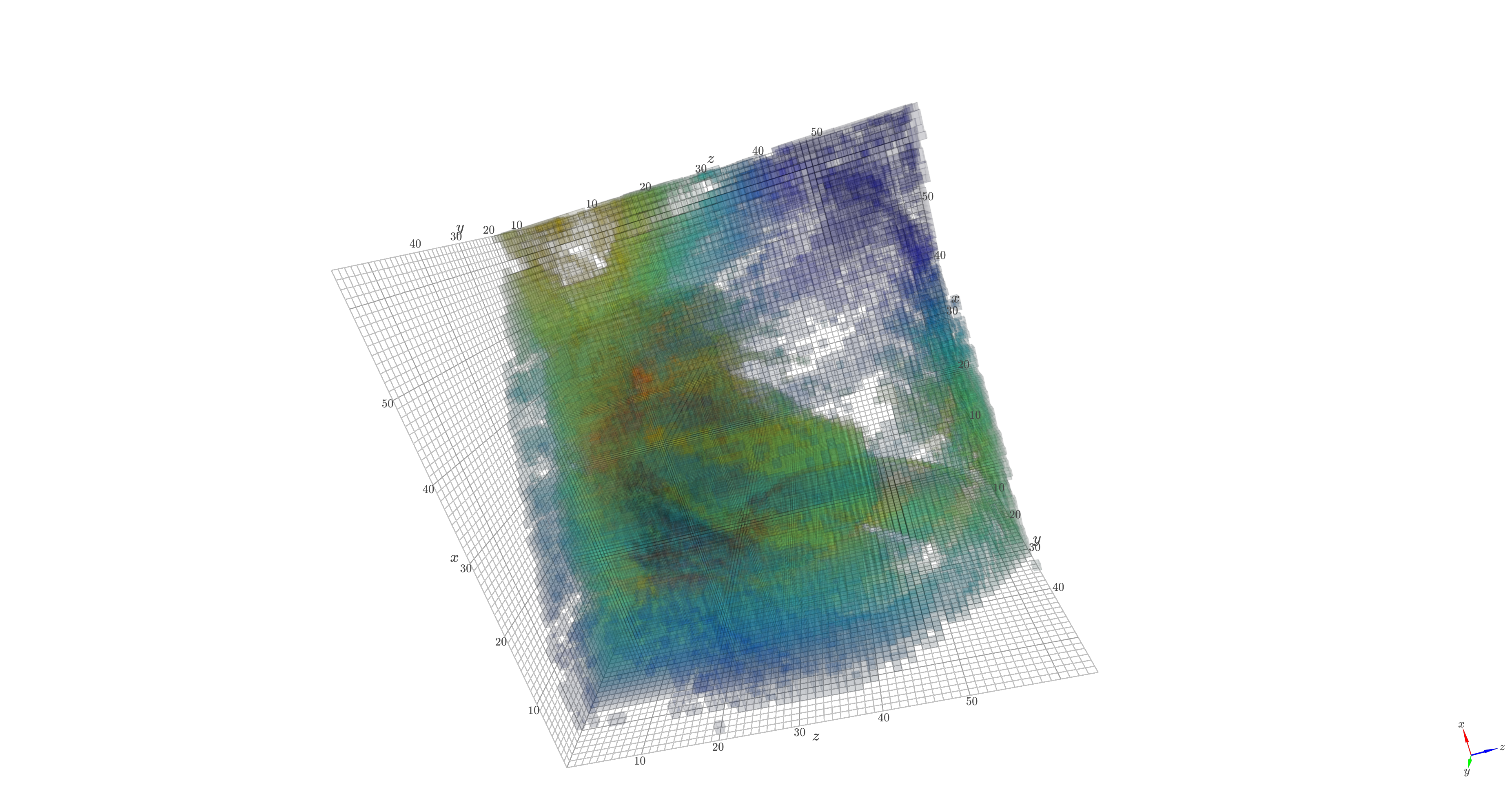
Generating Dermatoscopic Images With the Deep Energy-Based Model

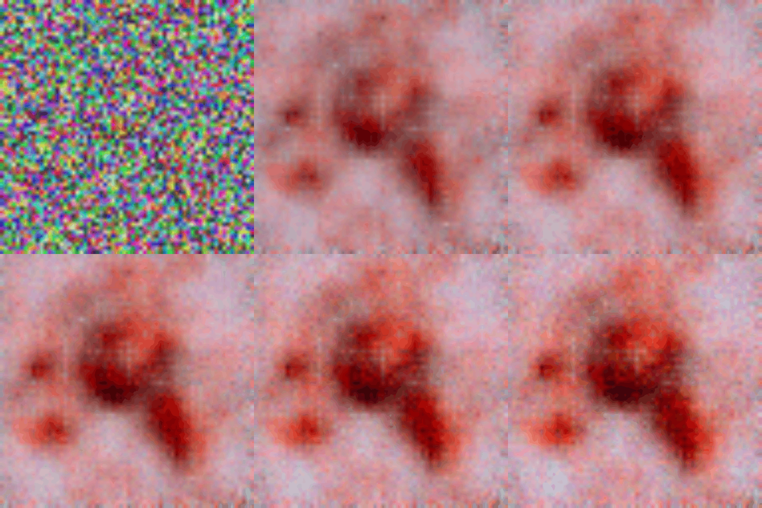
Transition from a random noise to a generated dermatoscopic image
Implicit generative models (e.g., diffusion models and GANs) are a promising avenue in which data generation bypasses the explicit restriction of adhering to the normalized data distribution. In the wake of deep learning, Energy-Based Models have jumped onto this path even harder. In the paper “Implicit Generation and Modeling with Energy-Based Models”, a deep learning model is used to model a negative energy function. The energy function defines the data probability distribution and an implicit generator by means of Langevin dynamics. It is optimized to assign low energy to real samples and high energy to generated ones. Next, the learned energy landscape is leveraged by Langevin dynamics for sample generation via stochastic gradient-based updates. The model is trained using contrastive divergence, comparing the energy of real images with that of synthetic samples initialized from noise (kind of similar to what Wasserstein GAN optimizes). The contrastive divergence stems from maximum likelihood estimation (MLE) of the data probability distribution. By doing so, we basically train a score-based model (reminiscent to diffusion models). Experimental results demonstrate that even a simple convolutional energy network can capture meaningful structure in medical image data and generate realistic dermatoscopic samples. It highlights the feasibility of applying EBMs in medical imaging and underscores their potential as a generative modeling tool in healthcare applications. This project’s source code is hosted on GitHub.
Generating Medical Images with the Label-Conditioned Latent Diffusion Model (From Scratch)
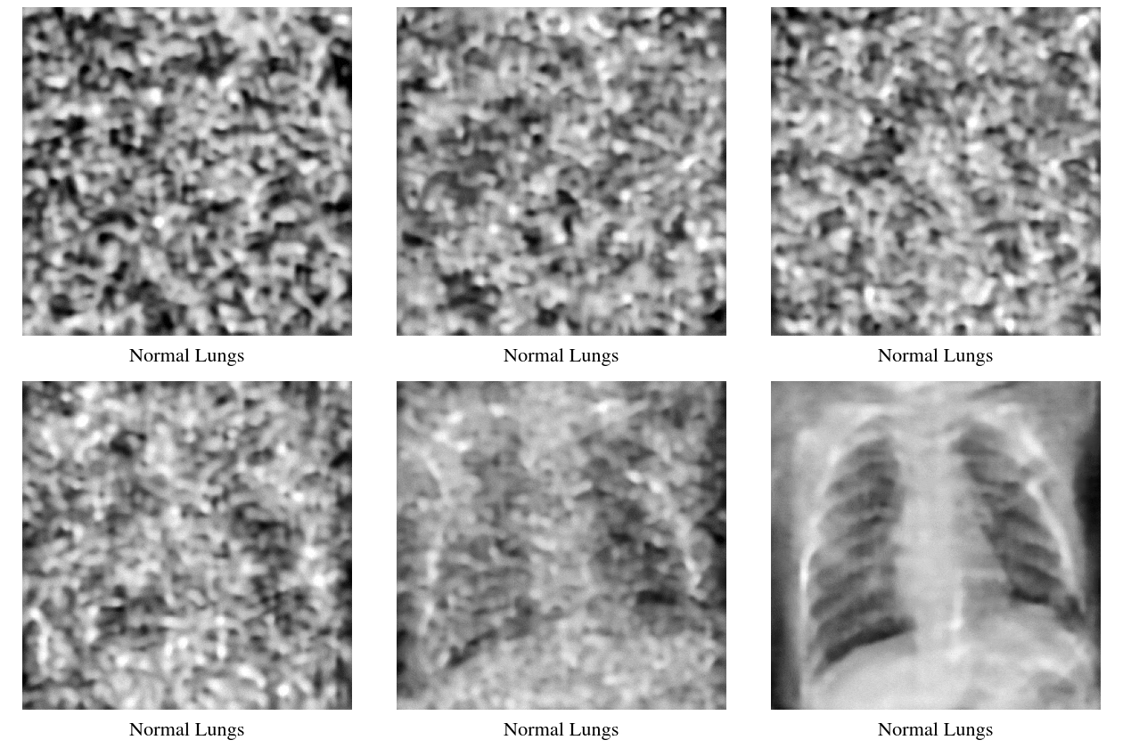 Label-conditioned generation of the normal chest X-ray
By 2021, we have witnessed the unprecedented feat of AI generating high-quality images and reshaping our digital world. We have reached this point thanks to a cutting-edge method: the latent diffusion model. This method is powered by prior research on VAE and diffusion models. Thus, out of curiosity, this project was done to realize the latent diffusion model from scratch. The VAE model employed in this project is VQ-VAE. DDPM is opted in for the diffusion model. Here, the PneumoniaMNIST dataset is used such that the latent diffusion model can generate chest X-ray images from random noise. Also, the generation is conditioned on labels: normal or pneumonia. Furthermore, to make the model more true to the label, we can adjust the value of the classifier-free guidance scale for better results. This project’s source code is hosted on GitHub.
MedBot: Medical Chatbot with Instruction Fine-Tuning and Conversational Memory
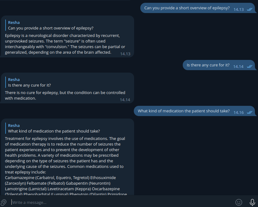 Conversation about Epilepsy with MedBot.
Language can be thought of as a conduit through which our abstract mind is exposed. Recently, the growth of AI has followed this notion, and almost everyone in the world benefits from it on a regular basis, particularly in the medical field. The language-based AI technology has the potential to alter the medical industry by allowing patients to connect with conversational machines. It allows anyone to get medical information from a computer in a more natural way. We can create a chatbot that plays the role of a medical practitioner. MedBot, a chatbot, is built on the well-known LLM, LLaMA 3, with instruction fine-tuning. It follows the directions in the prompt. To alleviate the effort of fine-tuning, the notoriously heavyweight LLM is quantized using 4-bit quantization. Additionally, LoRA (low-rank adaptation) is applied. These methods are collectively referred to as QLoRA. To maximize the fine-tuning efficiency, we have to load the LLM from the Unsloth library. Once the LLM model is fine-tuned, we can funnel it to LangChain, rendering a chatbot with conversational memory. We can converse with the chatbot via the Telegram bot. Last but not least, the fine-tuned LLM is trained and tested on Shekswess/medical_llama3_instruct_dataset_short. Finally, ROUGE is used to measure its quantitative performance. This project’s source code is hosted on GitHub.
Visualizing 3D ResNet for Medical Image Classification With Score-CAM
Intepretability is one of the concerns regarding the application of AI, or, to be exact, deep learning, in the medical field, especially medical image recognition. In a venture seeking to explain what is going on or what the network perceives computationally, one can leverage the class activation map (CAM) of the model. Score-CAM, one of the CAM variants, breakthroughs the preceding CAM methods by dropping the reliance on gradients. Instead, it benefits the full potential of the forward propagation of the model, running inference by normalized-weighting via element-wise product with the input. Then, the output logit of the target category is combined with the CAM acquired before to get the final outcome. In this project, the 3D version of ResNet is employed. To evaluate the aforementioned methods, the OrganMNIST3D dataset of MedMNIST is used. The deletion area under the curve (DAUC) and the insertion area under the curve (IAUC) are adopted to measure the performance of Score-CAM. This project’s source code is hosted on GitHub.
Medical Image Similarity Search Using a Siamese Network With a Contrastive Loss
 The image similarity search results for DermaMNIST (first row), PneumoniaMNIST (second row), RetinaMNIST (third row), and BreastMNIST (fourth row).
Obtaining the ontological account of an image numerically can be earned via a Siamese network. The anatomy of this network has a twin architecture, consisting of convolutional and fully connected layers with shared weights. Each architecture digests an image and yields the vector embedding (the ontological or latent representation) of that image. These two vectors are then subjected to the Euclidean distance calculation. Next, the result is funneled to the last fully connected layer to get the logit describing their similarity. To learn the representation, here, we can leverage contrastive loss as our objective function to be optimized. The network is trained on paired images, i.e., positive and negative. In this project, the positive pairs are two images that belong to the same dataset, and the negative pairs are two images from distinct datasets. Here, subsets of the MedMNIST dataset are utilized: DermaMNIST, PneumoniaMNIST, RetinaMNIST, and BreastMNIST. Then, accuracy is used to evaluate the trained network. Afterward, we encode all images of the train and validation sets into embedding vectors and store them in the PostgreSQL database. So, sometimes later, we can use the embedding vectors to retrieve similar images based on a query image (we can obtain it from the test set). To find similar images, FAISS (Facebook AI Similarity Search) is employed. FAISS helps us seek the closest vectors to the query vector. This project’s source code is hosted on GitHub.
Knowledge Distillation for Skin Lesion Classification
 The qualitative result of the distilled model.
The goal of knowledge distillation is to improve the performance of the half-witted model, which, most of the time, has fewer parameters, by allowing it to learn from the more competent model or the teacher model. The half-witted model, or the student model, excerpts the knowledge from the teacher model by matching its class distribution to the teacher model’s. To make the distributions softer (used in the training process as the part of the loss function), we can adjust a temperature T to them (this is done by dividing the logits before softmax by the temperature). This project designates EfficientNet-B0 as the teacher and SqueezeNet v1.1 as the student. These models will be experimented on the DermaMNIST dataset of MedMNIST. We will take a look at the performance of the teacher, the student (without knowledge distillation), and the student (with knowledge distillation) in the result section. This project’s source code is hosted on GitHub.
Medical Image Latent Space Visualization Using VQ-VAE
 The latent space of five distinct datasets, i.e., DermaMNSIT, PneumoniaMNIST, RetinaMNIST, BreastMNIST, and BloodMNIST.
In this project, VQ-VAE (Vector Quantized VAE) is leveraged to learn the latent representation z of various medical image datasets x from MedMNIST. Similar to VAE (Variational Autoencoder), VQ-VAE consists of an encoder q(z|x) and a decoder p(x|z). But unlike VAE, which generally uses the Gaussian reparameterization trick, VQ-VAE utilizes vector quantization to sample the latent representation z ~ q(z|x). Using vector quantization, it allows VQ-VAE to replace a generated latent variable from the encoder with a learned embedding from a codebook C ∈ RE × D, where E is the number of embeddings and D is the number of latent variable dimensions (or channels in the context of image data). Let X ∈ RH × W × D be the output feature map of the encoder, where H is the height and W is the width. To transform the raw latent variable to the discretized one, first we need to find the Euclidean distance between X and C. This step is essential to determine the closest representation of the raw latent variable to the embedding. The computation of this step is roughly expressed as: (X)2 + (C)2 - 2 × (X × C). This calculation yields Z ∈ RH × W, where each element denotes the index of the nearest embedding of the corresponding latent variable. Then, Z is subject to C to get the final discrete representation. Inspired by the centroid update of K-means clustering, EMA (exponential moving average) is applied during training, which updates in an online fashion involving embeddings in the codebook and the estimated number of members in a cluster. This project’s source code is hosted on GitHub.
Medical Image Generation Using Diffusion Model
 Unconditional progressive generation on the BloodMNIST dataset (left) and a montage of the actual BloodMNIST dataset (right).
Image synthesis on medical images can aid in generating more data for biomedical problems, which is hindered due to some legal and technical issues. Using the diffusion model, this problem can be solved. The diffusion model works by progressively adding noise, typically Gaussian, to an image until it is entirely undistinguishable from randomly generated pixels. Then, the noisy image is restored to its original appearance gradually. The forward process (noise addition) is guided by a noise scheduler, and the backward process (image restoration) is carried out by a U-Net model. In this project, the diffusion model is trained on the BloodMNIST dataset from the MedMNIST dataset. This project’s source code is hosted on GitHub.
Small Molecular Graph Generation for Drug Discovery
 The qualitative results of the generated molecules. The chemical structure, the SMILES representation, and the QED scores are provided.
With the advent of deep learning, drug development can be sped up just by learning the patterns within the molecules regarding their chemical properties and composition. The pursuit of good candidates for drugs can be achieved using the generative model which can extrapolate the unseen molecular structure. In this project, one of the most popular generative models, Generative Adversarial Network or GAN, is utilized. The generator of GAN consists of MLP, and the discriminator of GAN consists of R-GCN + MLP. Nowadays, there are plenty of open-sourced datasets that can be used for this purpose such as the QM9 (Quantum Machines 9) dataset. The GAN model is trained on QM9 dataset and its performances are assessed by means of molecular metrics, i.e., quantitative estimate of druglikeness (QED), solubility (defined as the log octanol-water partition coefficient or logP), synthetizability, natural product, drug candidate, valid, unique, novel, and diversity. This project’s source code is hosted on GitHub.
Self-Supervised Contrastive Learning for Colon Pathology Classification
 The qualitative result of the fine-tuned pre-trained SSL model.
Self-supervised learning, or SSL, has become a modern way to learn the hidden representation of data points. A dataset is not always provided with a label that marks a data point’s category or value. SSL mitigates this issue by projecting a data point into an embedding vector representing information beneath. SSL can be trained contrastively, i.e., to measure the similarity between two projected embeddings (original and augmented) using certain metrics, e.g., cosine similarity, Euclidean distance, Manhattan distance, etc. By learning the latent representation, the SSL model can be utilized as a pre-trained model and fine-tuned as needed. The SSL model is divided into three parts: the backbone feature extractor, the embedding projection head, and the classification head. The backbone feature extractor leverages ResNet 18. The embedding head gives the embedding vector. The classification head concludes the classification task’s result. Here, two other models are also introduced: the baseline model and the fine-tuned pre-trained SSL model. Both of them consist of a backbone feature extractor and a classification head. Yet, the latter makes use of the trained SSL model’s backbone as its own backbone. To evaluate the performance of the models, the PathMNIST of the MedMNIST dataset is utilized. On batched training, the other pairs in the batch relative to a certain pair (positive pair) are treated as negative pairs. This notion is useful for the computation of the contrastive loss: NTXentLoss/InfoNCE. This project’s source code is hosted on GitHub.
EEG Motor Imagery Classification Using CNN, Transformer, and MLP
 An illustration of the CNN-Transformer-MLP model.
The electroencephalogram, or EEG for short, is one of the biosignals that display brain activity in the form of time-series data. EEG can be used to help amputees or paralyzed people move their prosthetic arms via a brain-computer interface (BCI). In order to identify the correct limbs to control from the EEG signal, a combination of CNN, Transformer, and MLP is utilized in this work for motor imagery (MI) classification. CNN converts the epoched EEG signal into meaningful representation in accordance with the signal’s non-stationary nature. Transformer finds the global relationship of the given representation from CNN. MLP classifies the expected upper limbs to move based on the extracted information from the Transformer. To gauge the capability of the CNN-Transformer-MLP model, PhysioNet’s EEG Motor Movement/Imagery Dataset is used. The model attains an accuracy of 76.4% on the test set. This project’s source code is hosted on GitHub.
COVID19CT3D
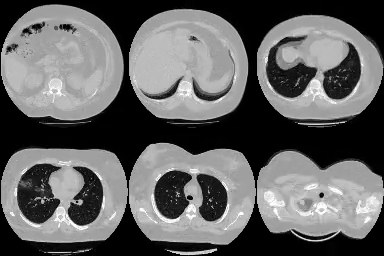
This tutorial will teach you how to train a Deep Learning model based on 3D Convolution. This model will classify whether the volumetric medical image from a 3D CT scan of the thorax is infected by COVID-19 or not. The model’s output is a single-valued tensor that represents the probability of being infected by COVID-19. This tutorial is based on A tutorial notebook on 3D image classification. This project’s source code is hosted on GitHub.
GGB
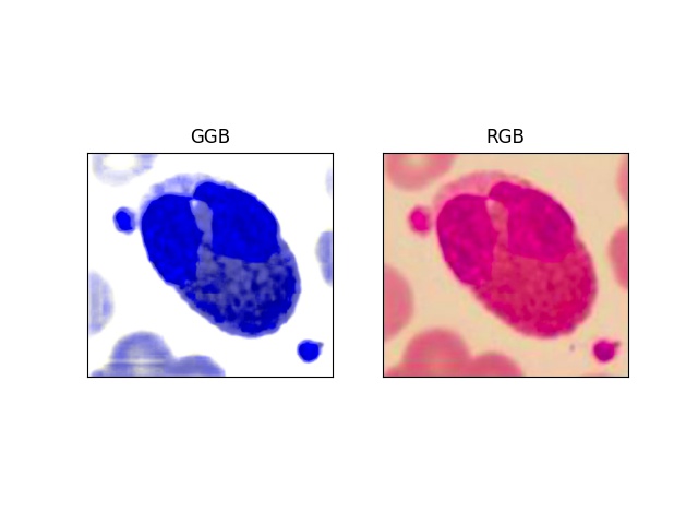
This package is implementation of GGB color space from Development of a Robust Algorithm for Detection of Nuclei and Classification of White Blood Cells in Peripheral Blood Smear Image. GGB’s source code is hosted on GitHub.
MyQLaNet
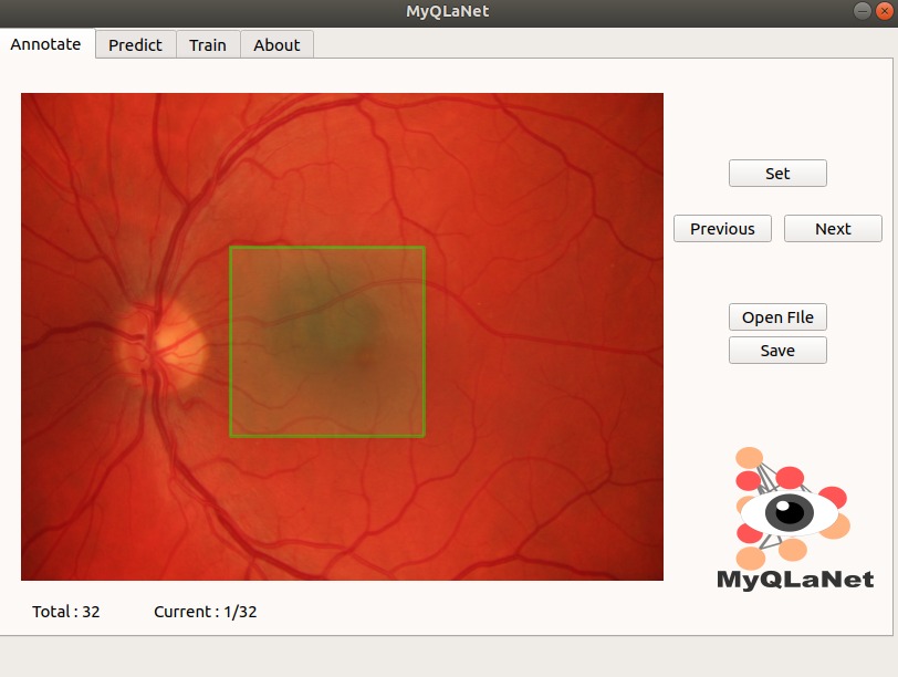
MyQLaNet is a Deep Learning platform for macula detection. It provides end to end system for macula detection with graphical user interface. MyQLaNet’s source code is hosted on GitHub.
Computer Vision
Exploring Latent Space via VAE
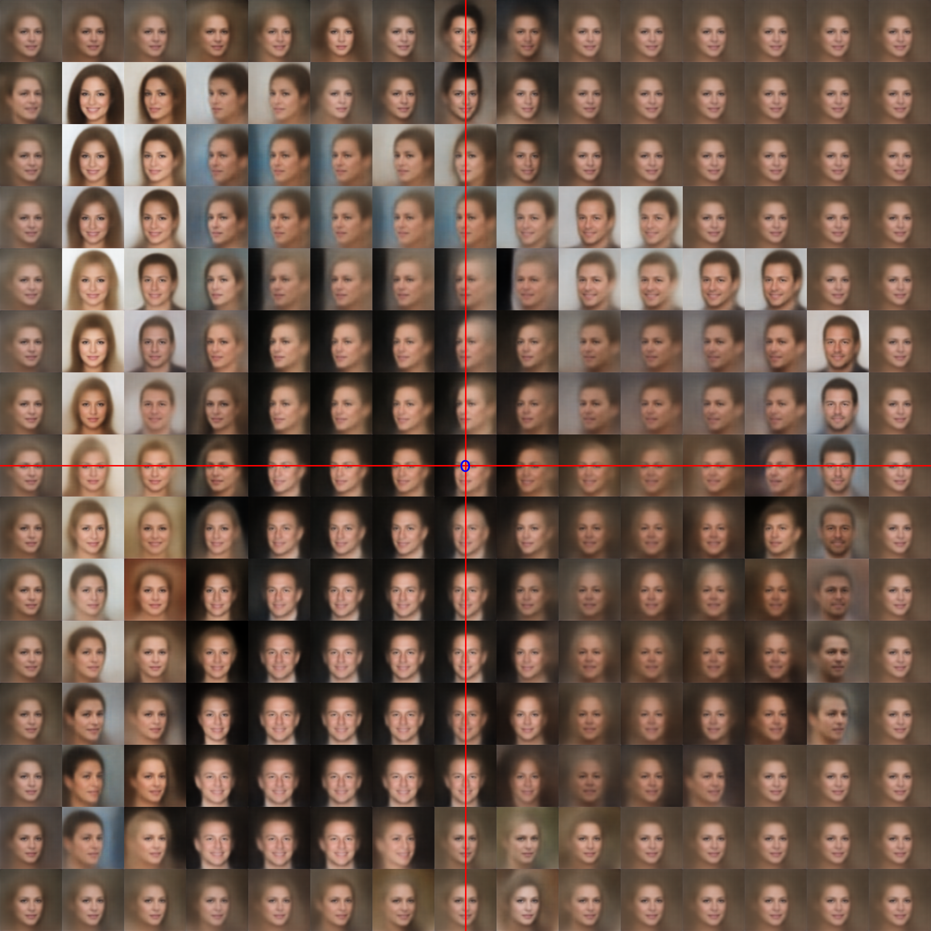
The 2D latent space in a 15 × 15 image grid
VAE and the latent space are the inseparable duo in representation learning. VAE uses the latent space as a constraint on how excellent data reconstruction should be. With a controlled latent space, we can simply regulate the data-generating process. On this occasion, we will go on an excursion across a latent space. We’ll see what we can do in this “Chamber of Secrets.” In the latent space, latent vectors (or variables) coexist harmoniously. Let’s see “Fantastic Latent Vectors and How to Find Them.” This project’s source code is hosted on GitHub.
Few-shot Learning with Reptile
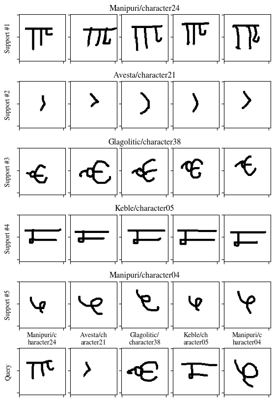 The top five rows contain support images. Each row indicates a separate class (or way). Each class has been provided with five shots (or samples) of images. The query images and their respective predicted classes are shown in the very bottom row.
Just by seeing an object several times, humans can identify it easily. This concept can be applied to artificial neural networks (ANNs) as well (i.e., few-shot learning). Meta-learning appears as a way to achieve this goal: an artificial neural network (ANN) must learn one of the learning components (e.g., optimizers, models, etc.) to behave with virtually the same level of adaptability as humans. The Reptile algorithm, one of the meta-learning techniques, makes sure the target model’s initial weights are appropriate for identifying provided inputs (like images) in minuscule quantities. The method follows the steps below for each epoch. Select a task (n selected classes with k data points each) at random from the dataset (for example, the Omniglot dataset). Use SGD or Adam to optimize the target model several times on the task. Shift the target model’s old weights to the direction of the new weights from the previous step. This project’s source code is hosted on GitHub.
Semi-Supervised Learning with Pseudo-Labeling
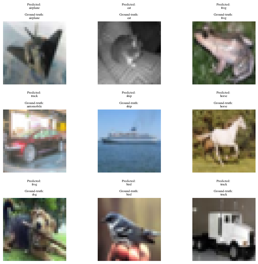 The grid of qualitative results.
The need for semi-supervised learning stems from the cost of annotating datasets. Datasets do not always come with fully labeled data. Henceforth, we can cleverly perform compound training with labeled and unlabeled data. One of the semi-supervised methods we can employ is pseudo-labeling. At first, we train our model with labeled data and generate labels for unlabeled data based on it. Next, we train the pre-trained model with both labeled and unlabeled data. This is possible due to pseudo-labels generated earlier. In this project, DenseNet-121 is utilized. The model is trained on CIFAR-10 with 1000 labels. This project’s source code is hosted on GitHub.
Instance Segmentation Using ViT-based Mask R-CNN
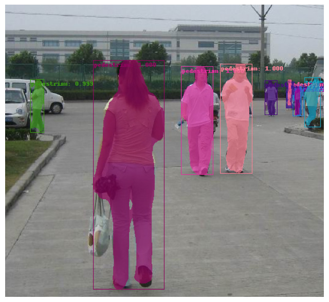 One of qualitative results from the ViT-based Mask R-CNN model.
Instance segmentation aims at dichotomizing a pixel acting as a sub-object of a unique entity in the scene. One of the approaches, which combines object detection and semantic segmentation, is Mask R-CNN. Furthermore, we can also incorporate ViT as the backbone of Mask R-CNN. In this project, the pre-trained ViT-based Mask R-CNN model is fine-tuned and evaluated on the dataset from the Penn-Fudan Database for Pedestrian Detection and Segmentation. With a ratio of 80:10:10, the train, validation, and test sets are distributed. This project’s source code is hosted on GitHub.
Domain Adaptation With Domain-Adversarial Training of Neural Networks
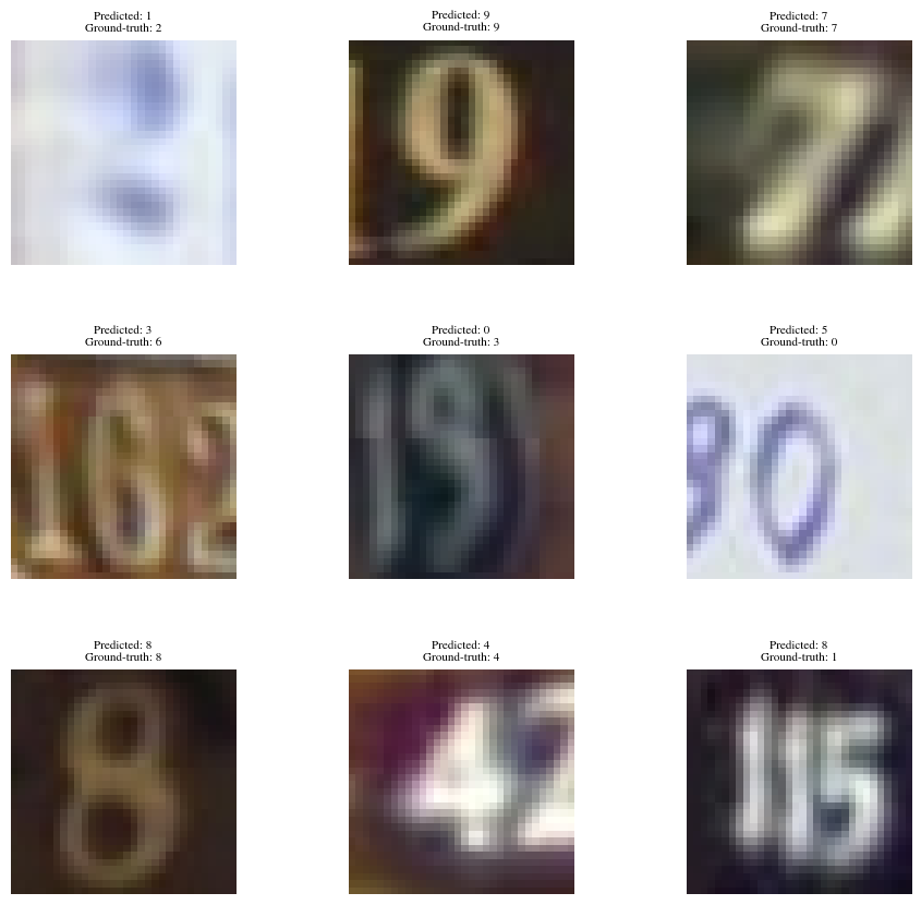 Some results on the SVHN dataset as the target dataset.
Domain adaptation’s main objective is to adapt the model trained on the source dataset in which the label is available to perform decently on the target dataset, which has a pertinent distribution yet the label is not already on hand. In this project, the pretrained RegNetY_400MF is leveraged as the model undergoing the adaptation procedure. The procedure is conducted with Domain-Adversarial Training of Neural Networks or DANN. Succinctly, DANN works by adversarially training the appointed model on the source dataset along with the target dataset. DANN uses an extra network as the domain classifier (the critic or discriminator) and applies a gradient reversal layer to the output of the feature extractor. Thus, the losses accounted for this scheme are the classification head loss (the source dataset) and the domain loss (the source dataset and the target dataset). Here, the source dataset is MNIST and the target dataset is SVHN. On MNIST, various data augmentations (geometric and photometric) are utilized on the fly during training. To monitor the adaptation performance, the testing set of SVHN is designated as the validation and testing set. This project’s source code is hosted on GitHub.
Image Classification With Vision Transformer
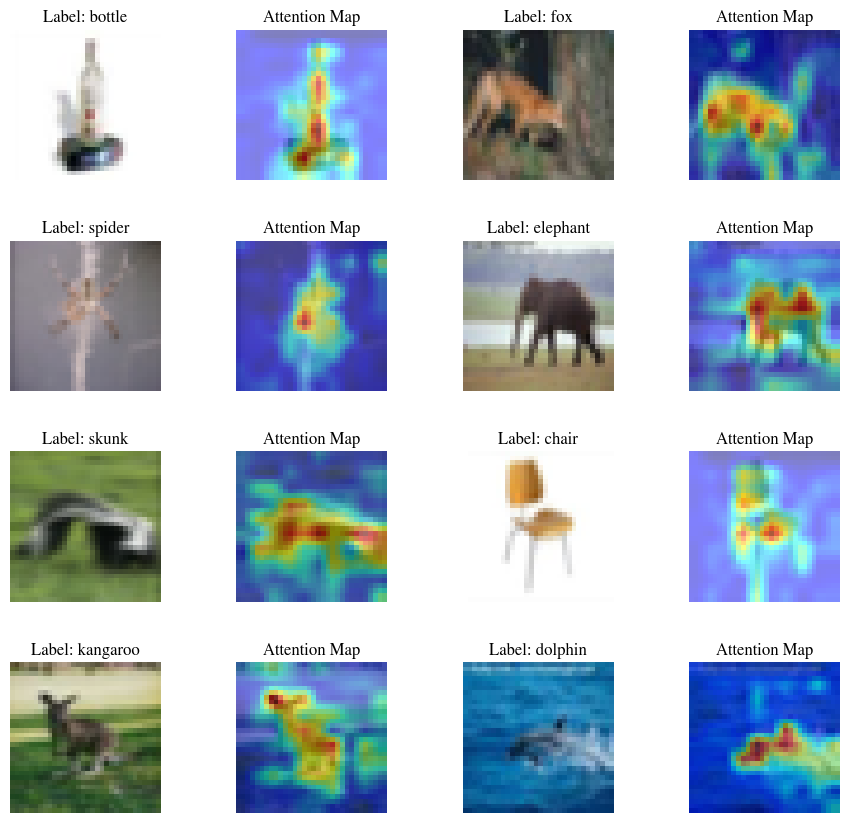 Several prediction results of ViT and their attention map.
Vision Transformer, or ViT, tries to perform image recognition in a sequence modeling way. By dividing the image into patches and feeding them to the revered model in language modeling, a.k.a. Transformer, ViT shows that over-reliance on the spatial assumption is not obligatory. However, a study shows that giving more cues about spatial information, i.e., subjecting consecutive convolutions to the image before funneling it to the Transformer, aids the ViT in learning better. Since ViT employs the Transformer block, we can easily receive the attention map explaining what the network sees. In this project, we will be using the CIFAR-100 dataset to examine ViT performance. Here, the validation set is fixed to be the same as the test set of CIFAR-100. Online data augmentations, e.g., RandAugment, CutMix, and MixUp, are utilized during training. The learning rate is adjusted by following the triangular cyclical policy. This project’s source code is hosted on GitHub.
Image Classification Using Swin Transformer With RandAugment, CutMix, and MixUp
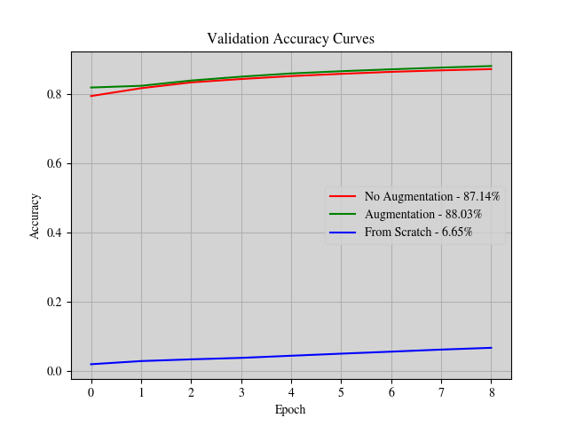 Accuracy curves of the models on the validation set.
In this project, we will explore three distinct Swin Transformers, i.e., without augmentation, with augmentation, and without using the pre-trained weight (or from scratch). Here, the augmentation is undertaken with RandAugment, CutMix, and MixUp. We are about to witness the consequences of utilizing augmentation and pre-trained weight (transfer learning) on the models on the imbalanced dataset, i.e., Caltech-256. The dataset is split per category with a ratio of 81:9:10 for the training, validation, and testing sets. For the from scratch model, each category is truncated to 100 instances. Applying the augmentation and pre-trained weight clearly boosts the performance of the model. Not to mention the pre-trained weight insanely pushes the model to effectively predict the right label in the top-1 and top-5. This project’s source code is hosted on GitHub.
Multi-Object Tracking Using FCOS + DeepSORT
![]() The result on KITTI-16.
The result on KITTI-16.
An idiot admires complexity, a genius admires simplicity…
― Terry Davis
As the term suggests, multi-object tracking’s primary pursuit in computer vision problems is tracking numerous detected objects throughout a sequence of frames. This means multi-object tracking embroils two subproblems, i.e., detection and tracking. In this project, the object detection problem is tackled via COCO dataset-pretrained FCOS, an anchor-free proposal-free single-stage object detection architecture. Meanwhile, the tracking problem is solved through the DeepSORT algorithm. To track each object, DeepSORT utilizes the Kalman filter and the re-identification model. The Kalman filter is widely used to predict the states of a certain system. In this case, the states are the pixel positions (cx, cy), the bounding box’s aspect ratio and height (w/h, h), and the velocity of cx, cy, w/h, and h of the objects. This project makes use of the simplified DeepSORT algorithm. The re-identification model aids in pinpointing two identical objects between frames based on their appearance. This model generates a vector descriptor associated with the objects in a frame. ImageNet-1K dataset-pretrained MobileNetV3-Small is leveraged as the backbone of the re-identification model. FAISS is set on duty in the matching process of an object’s appearance and pixel location in consecutive frames. Here, the datasets used for fine-tuning the re-identification model and evaluating the tracking are Market-1501 and MOT15, respectively. The train set of the MOT15 dataset is used for testing (producing the quantitative result) and the test set of the MOT15 dataset is used for inferencing (producing the qualitative result). This project sets the object to be tracked is the person. This project’s source code is hosted on GitHub.
Next-Frame Prediction Using Convolutional LSTM
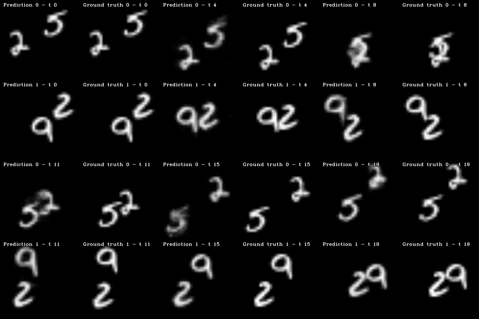
The Convolutional LSTM model predicts the ensuing frame-by-frame from t = 1 to t = 19.
In the next-frame prediction problem, we strive to generate the subsequent frame of a given video. Inherently, video has two kinds of information to take into account, i.e., image (spatial) and temporal. Using the Convolutional LSTM model, we can manage to feature-extract and process both pieces of information with their inductive biases. In Convolutional LSTM, instead of utilizing fully connected layers within the LSTM cell, convolution operations are adopted. To evaluate the model, the moving MNIST dataset is used. To evalute the model, the Moving MNIST dataset is used. This project’s source code is hosted on GitHub.
Point Cloud Segmentation Using PointNet
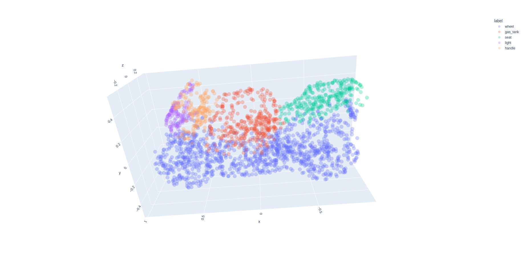 The segmentation result for the motorbike subcategory of the ShapeNet dataset with the labels: wheel, seat, gas_tank, light, and handle.
In this project, PointNet is leveraged for the segmentation of parts of a certain shape in the form of point cloud data. The data points are obtained from the ShapeNet dataset, i.e., ShapeNetCore. This project chooses the shape of a motorbike. PointNet is utilized due to its nature, which is invariant to permutation. Keep in mind that point cloud data has zero care for the spatial relationship between points in the point cloud, even though it stores information regarding the object’s location in the space. In other words, the order of points must be negligible and not influence the result. This project’s source code is hosted on GitHub.
Action Recognition Using CNN + Bidirectional RNN
 The action recognition results of the CNN + Bidirectional RNN model. Several actions are shown in the compilation video: brush hair, throw, dive, ride bike, and swing baseball.
Given a video, we can undergo recognition or analysis to decide what action occurred in the clip. By nature, videos are a sequence of frames. Consequently, performing action recognition on video deals with processing spatio-temporal data. Here, we can make use of the HMDB51 dataset, consisting of 6k+ clips of 51 actions. This dataset has three separate train/test splits. Striving for simplicity, this project utilizes the first training split as the training set, the second testing split as the validation set, and the third testing split as the testing set. Regarding the action recognition model, CNN is customarily adopted to extract spatial information. Thus, a CNN architecture, MnasNet, is put into use. Next, to handle the temporal information, bidirectional RNN is employed. Succinctly, the action recognition model in this project is composed of CNN and bidirectional RNN. This project’s source code is hosted on GitHub.
Novel View Synthesis Using NeRF
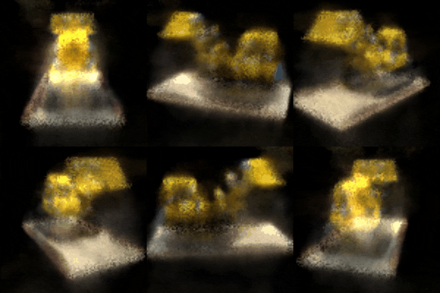 The rendered 3D view of a bulldozer viewed from x = 0, y = 0, z = 3.5, ϕ = −15°, and θ = 0° to 360°.
Legend has it that the artificial neural network (ANN) is infamously known as the universal approximator, which can fit any existing function. By exploiting this fact, we can build a network that approximates a function that maps spatial positions (x, y, z) and camera rays (these rays are acquired through the calculation of the camera matrix involving viewing directions (θ (rotating along the y-axis), ϕ (rotating along the x-axis)) and the spatial positions) to RGB pixels. Such a network, called the Neural Radiance Field, or NeRF in short, can be used to solve the problem of novel view synthesis of a scene. The network is coerced to overfit the function, which generates an RGB image (and also a depth map). These generated images (the final images are procured by computing the transmittance that is applied to the freshly generated images) from multiple angles are then collected, rendering the 3D representation of a certain object. In this project, a bulldozer from the Tiny NeRF dataset is used. This project’s source code is hosted on GitHub.
Image Super-Resolution Using ESRGAN
 Qualitative comparison between the reference high-resolution images (left column), high-resolution images via bicubic interpolation (middle column), and predicted high-resolution images through ESRGAN (right column).
Image super-resolution attempts to produce pixels within the image to fill the lack of information due to its low-resolution nature. Hence, it yields a higher-resolution image. One approach to this problem is via generative networks, e.g., ESRGAN (Enhanced Super-Resolution Generative Adversarial Network). This type of GAN is built explicitly for image super-resolution by considering several losses, i.e., contextual loss (focus on the distribution of the feature), perceptual loss (pixel-wise loss), and adversarial loss. These three losses are utilized for the generator loss. On the contrary, the discriminator loss only takes into account the adversarial loss. There are two stages during training: (1) train only the generator on the perceptual loss, and (2) train the generator and discriminator based on those, as mentioned earlier. The model is trained and evaluated on the BSDS500 dataset. The final result of the predicted high-resolution image is subjected to the sharpening method by subtracting the image with the Laplacian of the image. This project’s source code is hosted on GitHub.
Zero-Reference Low-Light Image Enhancement


 The qualitative results of the image enhancement method (comparing the original, the ground-truth, the PIL autocontrast, and the prediction).
Low-light image enhancement aims to raise the quality of pictures taken in dim lighting, resulting in a brighter, clearer, and more visually appealing image without adding too much noise or distortion. One of the state-of-the-art methods for this computer vision task is Zero-DCE. This method uses just a low-light image without any image reference to learn how to produce an image with higher brightness. There are four loss functions crafted specifically for this zero-reference low-light image enhancement method, i.e., color constancy loss, exposure loss, illumination smoothness loss, and spatial consistency loss. This project’s source code is hosted on GitHub.
Anchor-Free Object Detection
 Two motorbikes (left), a person and a horse (middle), and a car and an aeroplane (right) are detected.
Anchor boxes have been the prevalent way to generate candidates for the ground truth bounding boxes in the object detection problem. Yet, this approach is such a hassle and downright confusing. This tutorial leverages an object detection method named FastestDet that is lightweight and anchor-free. PASCAL VOC 2007 and 2012 datasets are utilized to evaluate the model’s capability. Here, the train and validation sets of PASCAL VOC 2012 are used for the train and validation while the test set of PASCAL VOC 2007 is allotted for the testing phase in this tutorial. Eventually, the inference set (the test set of PASCAL VOC 2007) is used to see the qualitative performance of the model. This project’s source code is hosted on GitHub.
Stable Diffusion Dreaming
Generate video by stable diffusion in Colab Notebook. This project’s source code is hosted on GitHub.
Image Captioning API

Minimal implementation of image captioning API hosted on Heroku. It receives an image and responds with a caption regarding the image. This project’s source code is hosted on GitHub.
SotoDemoBot

Simple Object detection Telegram bOt DEMO: predict the objects in the given image. Use /predict <URL> to predict the objects in the image of given url. This project’s source code is hosted on GitHub.
Natural Language Processing
Masked Language Modeling with BERT in Multi-GPU Settings
Input sentence: Please [MASK] [MASK] [MASK] [MASK] [MASK] [MASK]!
Top 5 predictions:
  Token: 'it' | Score: 0.4329 | Sequence: 'please stop the war. stop it!'
  Token: 'this' | Score: 0.2217 | Sequence: 'please stop the war. stop this!'
  Token: 'fighting' | Score: 0.0610 | Sequence: 'please stop the war. stop fighting!'
  Token: 'us' | Score: 0.0407 | Sequence: 'please stop the war. stop us!'
  Token: 'them' | Score: 0.0325 | Sequence: 'please stop the war. stop them!'
An example of a masked input sentence and its unmasked sentences generated by BERT.
This project demonstrates how to train a masked language model using BERT in a multi-GPU environment on Kaggle. The training process is powered by HuggingFace’s transformers and accelerate libraries, making distributed training seamless and accessible. The model is fine-tuned on the Wikitext dataset provided by Salesforce. This project’s source code is hosted on GitHub.
GPT2Chat: Creating a GPT-2-Based Chatbot with Human Preferences
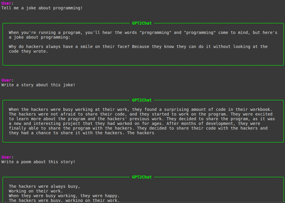
A sample of conversation with GPT2Chat on Colab.
In this project, a conversational chatbot named GPT2Chat, based on the GPT-2 language model, is developed. To enable the model to engage in meaningful dialogues, first, instruction fine-tuning is performed using the OpenAssistant Conversations Dataset (OASST1) and the Alpaca dataset. The LLaMA3 instruction template is adopted and adapted by incorporating special tokens <|start_context|> and <|end_context|> to encapsulate conversation history, thereby providing contextual awareness to the model. Subsequently, the ORPO method is employed for preference alignment, utilizing the trl-lib/ultrafeedback_binarized dataset to refine the model’s responses based on human feedback. The resulting chatbot demonstrates decent conversational capabilities, leveraging both fine-tuning and preference learning techniques. This project’s source code is hosted on GitHub.
Instruction Fine-tuning of the GPT2MoE Model: GPT-2 with Mixture-of-Experts
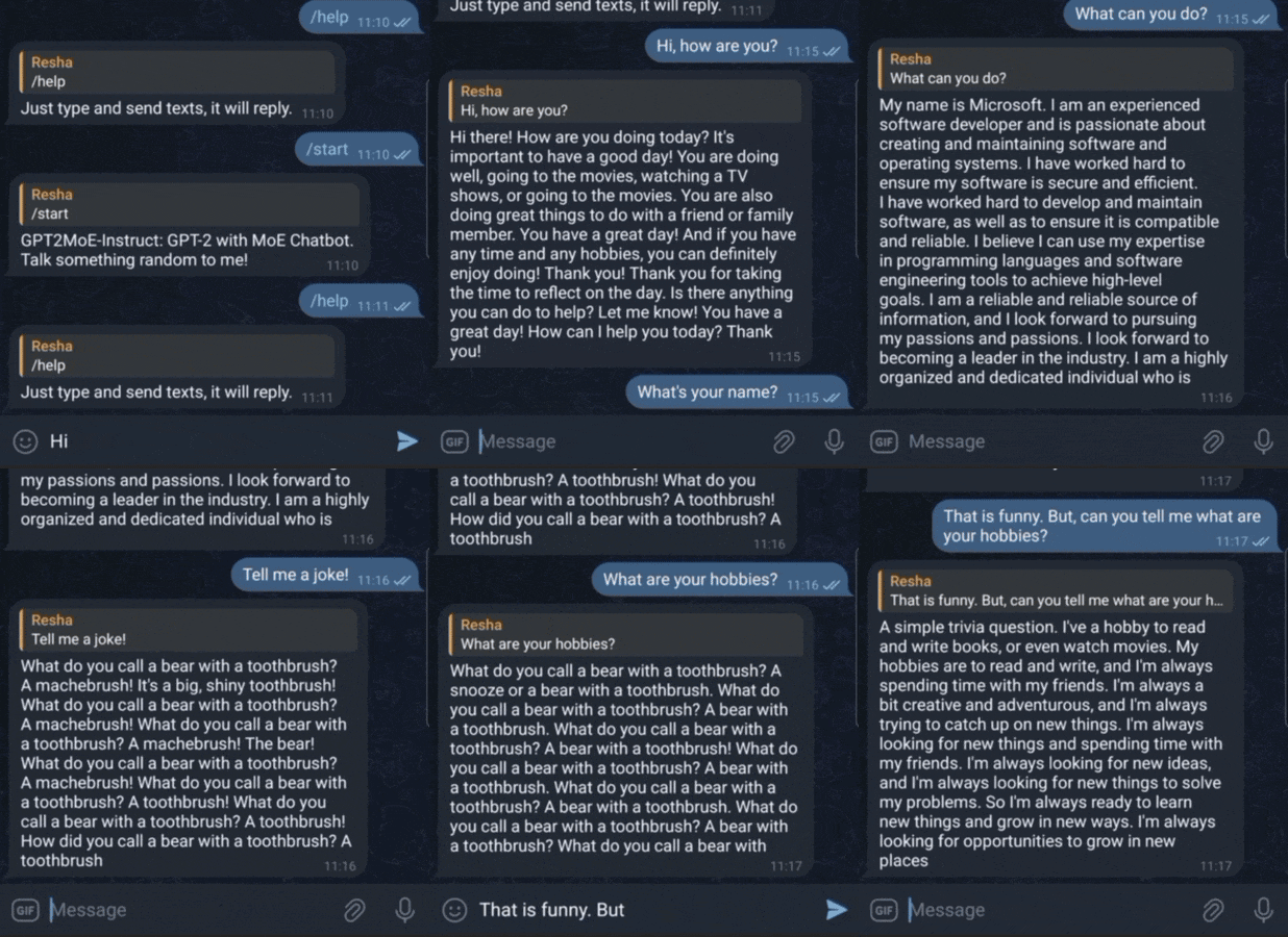
Conversing with GPT2MoE via Telegram Bot. It has conversational ability thanks to LangChain.
Large Language Models (LLMs) have demonstrated remarkable capabilities in various natural language processing tasks. This project presents GPT2MoE, a pre‐trained GPT-2 model with Mixture-of-Experts (MoE) layers, replacing its original feed-forward networks with FFNSwiGLU-based experts. This project employs a transfer learning strategy where the original GPT-2 weights are initialized by loading the pre-trained weights, while the weights of the newly introduced MoE layers are trained from scratch. The model is then instruction fine-tuned on the Stanford Alpaca instruction‐tuning dataset using state-of-the-art frameworks, HuggingFace for model handling and PyTorch Lightning for the training infrastructure. This report details the model architecture, the transfer learning and fine-tuning methodology, and presents the experimental results. This project’s source code is hosted on GitHub.
RAG-Bot: Chatbot with RAG
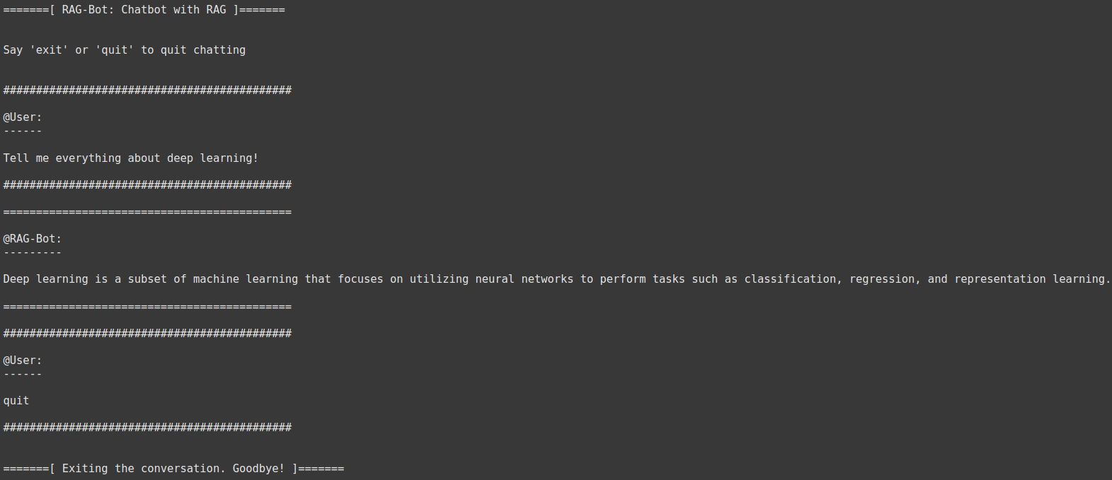 Conversation with RAG-Bot.
RAG-Bot is a minimalist chatbot built under the RAG (Retrieval-Augmented Generation) edifice. It employs GPT-2 as the generator model, fine-tuned on the open-instruct-v1 dataset. The retrieval process embroils several Wikipedia articles pertaining to AI. Later, the articles are chunked into sentences and subjected to SentenceTransformers, obtaining vector embeddings. The most relevant sentences are then augmented to enhance the user’s prompt. Owing to the LangChain framework, this bot performs RAG while conversing with the user seamlessly. This project’s source code is hosted on GitHub.
Question-Answering using GPT-2’s PEFT with LoRA
 Testing the model on a Winograd schema question.
Having constrained resources, the most rational way to fine-tune the language model with many parameters is to perform PEFT (parameter-efficient fine-tuning). One of the preferred PEFT methods is LoRA (low-rank adaptation). LoRA can decompose a complex neural network matrix (W) into two smaller matrices (A × B). These matrices are leveraged to re-parameterize the frozen weight of the language model (y = (W + A × B) × x). In this fashion, we can fine-tune the model inexpensively. In this project, we use GPT-2 as the baseline model. Then, LoRA is applied to the attention and linear layers. We fine-tune the model to carry out the question-answering task on the SQuAD 2.0 dataset. Next, the model is evaluated with BLEU 1-gram. The model, LoRA, dataset, and evaluation are available thanks to the Hugging Face ecosystem. This project’s source code is hosted on GitHub.
Image Captioning With MobileNet-LLaMA 3
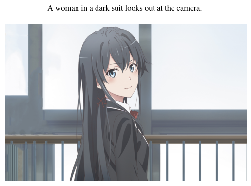 The result of MobileNet-LLaMA 3 in the wild.
Image captioning is one of the problems in computer vision, constituting two kinds of modalities, i.e., image and text. Given a particular image, a caption regarding it is automatically generated. One can easily leverage a CNN-based architecture to draw the numerical representation out of the image. When interacting with the text, the long-range dependencies method has to be employed. Uplifted by the recent success of LLaMA 3, this project utilizes its computational block called the LLaMA 3 Transformer block. This block comprises RMSNorm, Grouped Multi-Query Attention, Feed Forward SwiGLU, and Rotary Position Embedding. Anyhow, in the original implementation, the Transformer block was only used as the decoder. In this project, the Transformer block is used as both the encoder and the decoder. In the encoder, before image data is funneled into the architecture, a CNN-based architecture, MobileNet-V3, is leveraged, acting similarly to the text embedding. Therefore, this architecture is dubbed MobileNet-LLaMA 3. To get knowledge on the performance of the model, the Flickr-8k dataset is used. The dataset is separated into the train, validation, and test sets in the 80-10-10 rule. Quantitatively, the performance of the model is measured via the ROUGE score, to be precise, the ROUGE-1 F-measure. This project’s source code is hosted on GitHub.
Visual Question Answering Using CLIP + LSTM
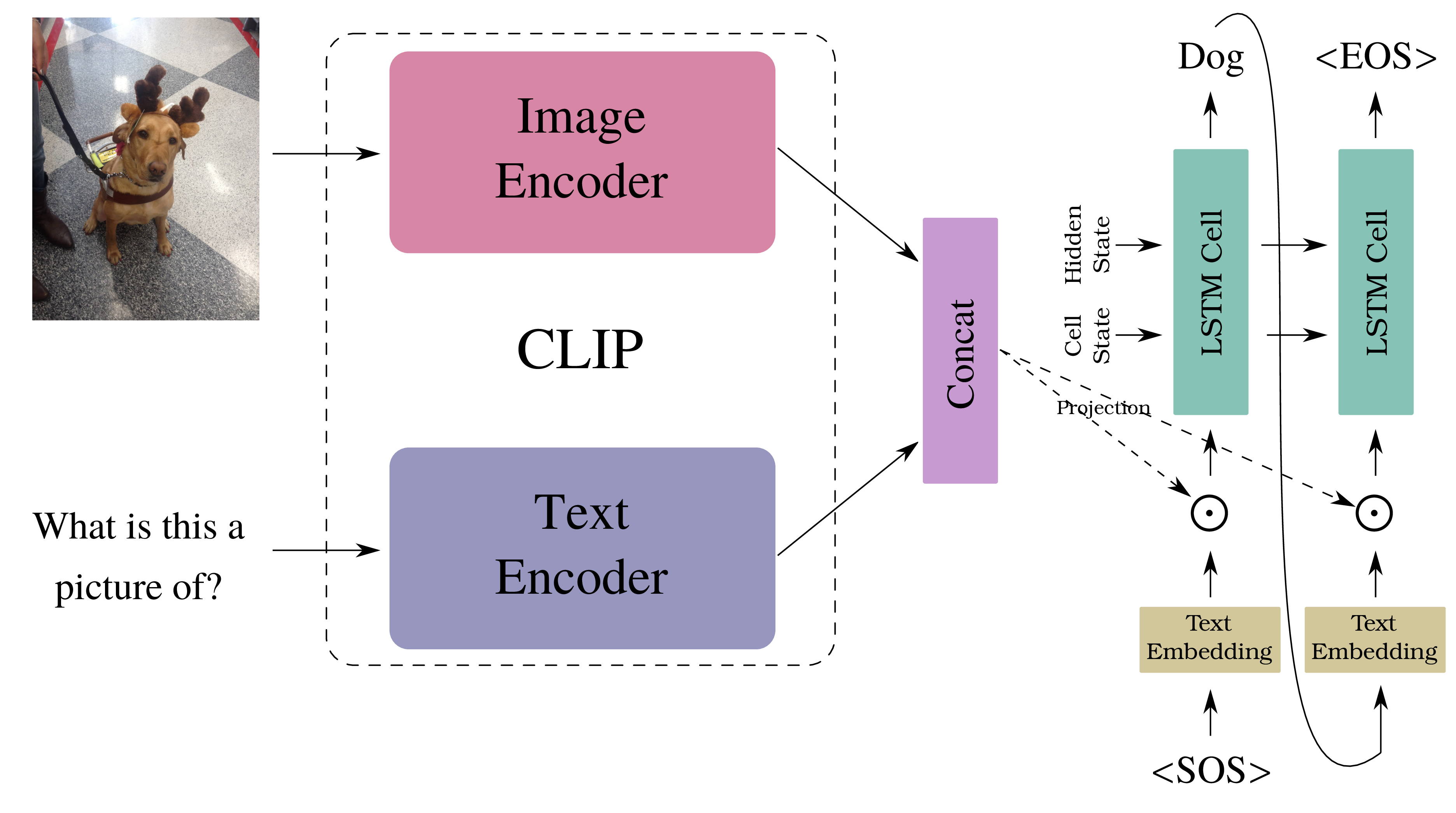 CLIP + LSTM architecture.
The visual question-answering problem can be described as “asking our computer to reply to the assigned questions about a particular image.” In this project, a CLIP + LSTM architecture comes to lend a helping hand, trying to solve the problem. The image and text encoders of CLIP cultivate the given image and question, respectively. The concatenated image-text representation from CLIP is then applied to the vectorized answer text via the Hadamard product before feeding it to LSTM. By a fashion of autoregressive, the answer to the question is finally served to us. Here, the VizWiz-VQA dataset is utilized to train, validate, and test the model. The training set of the dataset is used in the training and validation phases. It is divided by a ratio of 99:1. The validation set of the dataset is employed for testing. The SQuAD and BLEU metrics are utilized to gauge the performance of the model quantitatively. In inference time, the test set of VizWiz-VQA is leveraged. This project’s source code is hosted on GitHub.
English-To-German Neural Machine Translation Using Transformer
 The attention maps from each of the Transformer's heads. Almost every corresponding word pair (English-German) at each head pays attention mutually.
Neural Machine Translation (NMT) is a family model or an approach to solving machine translation problems through an artificial neural network, typically deep learning. In other words, the model is dispatched to translate a sequence of words from the source language to the target language. In this case, the source language would be English and the target would be German. To fabricate the model, the Transformer layers are leveraged. The NMT model is trained on the Multi30K dataset. The model is then assessed on a subset of the dataset, which is the Flickr 2016 test dataset. This project’s source code is hosted on GitHub.
Movie Review Sentiment Analysis Using CNN and MLP
 Visualization of the first layer of CNN on the negative review.
Audiences’ reactions to the movie they have watched can be presented in a text format called reviews. These reviews can be polarized into two clusters: positive responses and negative responses. Using CNN and MLP, one can perform sentiment analysis on movie reviews to automatically recognize the viewer’s tendency toward a particular movie. CNN is used for extracting the latent information within the text format. MLP leverages the extracted information and carries out the classification task. The CNN-MLP model is evaluated with Standford’s IMBD Movie Review dataset. On the test set, the model achieves 85.6% accuracy. This project’s source code is hosted on GitHub.
Your Kind Friend Bot: Unreliable Chatbot

Your typical kind friend who talk nonsense just to kill time. It can respond to text or image. Visit here. This project’s source code is hosted on GitHub.
Audio Data
AI Cover Song
Cover your favorite song by your favorite singer. This project’s source code is hosted on GitHub.
Music Genre Classification

Classify input audio into a particular genre of music. First, the audio is preprocessed via MFCC. Next, using MLP, we obtain the probability distribution of 10 classes of music genres. Before applying MLP to the MFCC, the cepstral coefficients with the length of the number of sequence of time has to be averaged and subjected to CMVN. This project’s source code is hosted on GitHub.
Graph Data
Web Traffic Prediction via Temporal Graph Neural Network
 The visitor prediction at one of the vital mathematics articles on Wikipedia.
Temporal Graph Neural Network or Temporal GNN is one of the variants of the GNN which handles the spatio-temporal data. The term “spatio-“ refers to the nature of the graph that is closely related to the spatial relationship that exists in the image data (recall that an image is basically a graph), and the term “temporal” here indicates the data may be progressively changing in a sequence of time. In this project, the Chebysev GCNN+LSTM module and the Wiki Maths dataset are leveraged, which are provided by PyTorch Geometric Temporal. The complete Temporal GNN model contains the Chebysev GCNN+LSTM module, followed by a fully connected layer. Here, the model is trained to predict the daily user visits to Wikipedia’s vital mathematics articles (represented by nodes/vertices). The graph’s characteristic in the dataset is non-heterogenous and static. The details of the dataset can be seen here. This project’s source code is hosted on GitHub.
Graph Neural Network for Node Classification
 The visualization of the embedding space of the nodes in the large graph in the course of the training process.
A graph neural network (GNN) is a type of neural network leveraged to handle graph data. One kind of graph data is a single graph that is large enough to contain a myriad of nodes. Later, we can attribute each node to well-qualified features and discriminate them accordingly. Then, by means of GNN, we can perform node classification on this large graph. The CORA dataset, the publicly available dataset for node classification on a large graph, is used in this tutorial. The graph feature extractor utilized in this tutorial consists of a sequence of ResGatedGraphConv, SAGEConv, and TransformerConv, which are implemented by PyTorch Geometric. The final classifier comprises MLP. This project’s source code is hosted on GitHub.
Machine Learning
PyTorch Depthwise Separable Convolution

PyTorch (unofficial) implementation of Depthwise Separable Convolution. This type of convolution is introduced by Chollet in Xception: Deep Learning With Depthwise Separable Convolutions. This package provides SeparableConv1d, SeparableConv2d, SeparableConv3d, LazySeparableConv1d, LazySeparableConv2d, and LazySeparableConv3d. This package’s source code is hosted on GitHub.
Neural Network

A naive implementation of a neural network. The code structure is heavily inspired by PyTorch and TensorFlow. However, this package is used for educational purposes and is not intended to be adopted in production. This project’s source code is hosted on GitHub.
Robotics
Balancing Act: Mastering the Inverted Double Pendulum with Soft Actor-Critic
These are the evolution of the control of the inverted double pendulum. The control is progressively better.
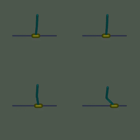 Episode 0
|
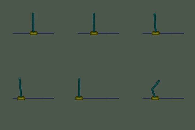 Episode 400
|
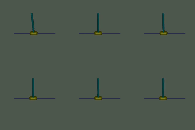 Final Episode
|
The inverted double pendulum is a hallmark of control theory, renowned for its instability and nonlinear dynamics. This project explores the challenge of stabilizing this system using the Soft Actor-Critic (SAC) algorithm, a state-of-the-art reinforcement learning method, within the MuJoCo physics engine. Through empirical experimentation, we harness SAC to develop a robust control strategy that balances the double pendulum upright with minimal torque, effectively navigating its complex behavior. Simulation results highlight SAC’s capability to adaptively learn policies for this demanding task, offering practical insights into its application for continuous control problems. This project demonstrates the power of SAC in addressing intricate dynamical systems and contributes to the growing field of reinforcement learning in control theory. This project’s source code is hosted on GitHub.
Teaching a Cheetah Robot to Run: Solving Continuous Control in Simulated Locomotion with Proximal Policy Optimization
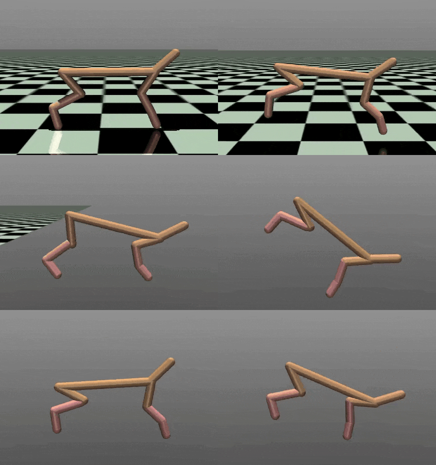 The Cheetah robot sprints predominantly stable in the simulated environment following the learned deterministic policy of PPO.
This project tackles the challenge of training a simulated Cheetah robot to run efficiently using reinforcement learning, focusing on the complexities of continuous action control. This project employs Proximal Policy Optimization (PPO), a stable and effective policy gradient algorithm, implemented with PyTorch, MuJoCo for realistic physics simulation, and Gymnasium as the environment framework. The policy and value networks, structured as multi-layer perceptrons, model actions via a Gaussian distribution, refined through iterative training with a clipped objective and Generalized Advantage Estimation (GAE) for stability. Key hyperparameters are tuned to optimize performance, and a deterministic policy—using the mean action—is adopted during evaluation to ensure consistency in the deterministic MuJoCo setting. The result is a Cheetah robot that achieves stable, agile locomotion with rising rewards, offering insights into continuous control and potential applications for real-world robotics. This project’s source code is hosted on GitHub.
Swinging Up Acrobot with n-Step Q-Learning
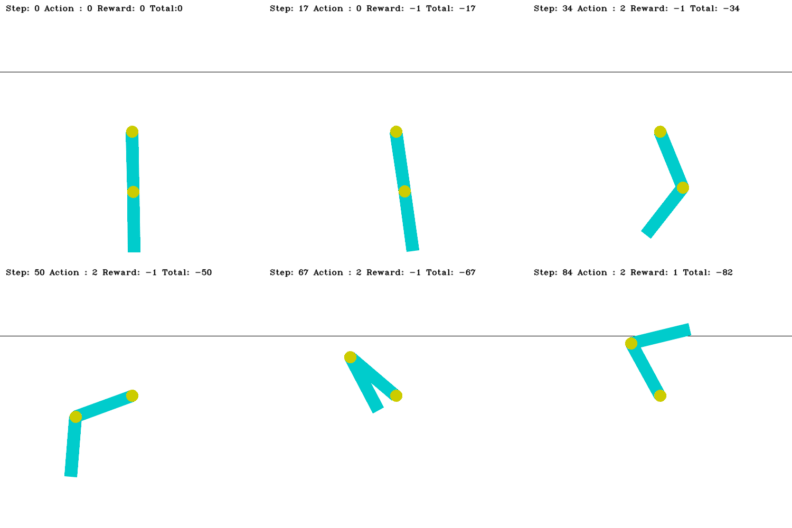 Acrobot's main challenge: set the last link above the horizontal threshold line as quickly as possible.
The Acrobot is a robotic arm with two links vertically suspended against gravity. It is an underactuated robot, and we can only exert torque on its elbow. Our goal is to raise its last link above a specified height indicated by a horizontal line. To fulfill this objective, we can use the n-step Q-learning algorithm, one of the family of TD(n) algorithms. TD(n) is a multi-step extension of TD learning (e.g., Q-learning). In the context of the Acrobot, the n-step Q-learning algorithm learns to select optimal actions (applying torque at the elbow) based on the current state (joint angles and velocities) and the expected future rewards. We could design the reward function to provide positive rewards for reaching the target height and penalties for inefficient movements or exceeding time limits. TD(n) uses the rewards collected over the next n steps plus the discounted Q-value at the n-th step instead of updating the Q-value based on just the immediate reward and the next state’s Q-value (as in TD(0) or the standard TD learning). This multi-step approach allows for better credit assignment over longer horizons, potentially speeding up learning. This project’s source code is hosted on GitHub.
Rocket Trajectory Optimization Using REINFORCE Algorithm
 The rocket successfully landed on the surface of the moon after hovering under the control of the learned policy from the REINFORCE algorithm.
In the context of machine learning, reinforcement learning (RL) is one of the learning paradigms involving interaction between agent and environment. Recently, RL has been extensively studied and implemented in the field of control theory. The classic example of a control theory problem is trajectory optimization, such as for spacecraft or rockets. Here, in the RL lingo, a rocket can be treated as an agent, and its environment would be outer space, e.g., the surface of the moon. The environment obeys the Markov Decision Process (MDP) property. The agent obtains a reward and observes a state based on the action that is given to the environment. The action taken by the agent is determined by the policy distribution that can be learned in the course of the training process. To learn the policy, one approach is to utilize the REINFORCE algorithm. This method is a policy gradient algorithm that maximizes the expected return (reward), incorporating Monte Carlo approximation. In practice, the expected return will be our objective function, applying the log-derivative trick to the trajectory probability to update our policy distribution. This project’s source code is hosted on GitHub.
Suction Arm Manipulator Robot
Simulate the Suction Arm Manipulator Robot to pick up daily objects inspired by the Amazon Robotics Challenge. This project’s source code is hosted on GitHub.
Quantum Machine Learning
Image Recognition with Quantum LeNet
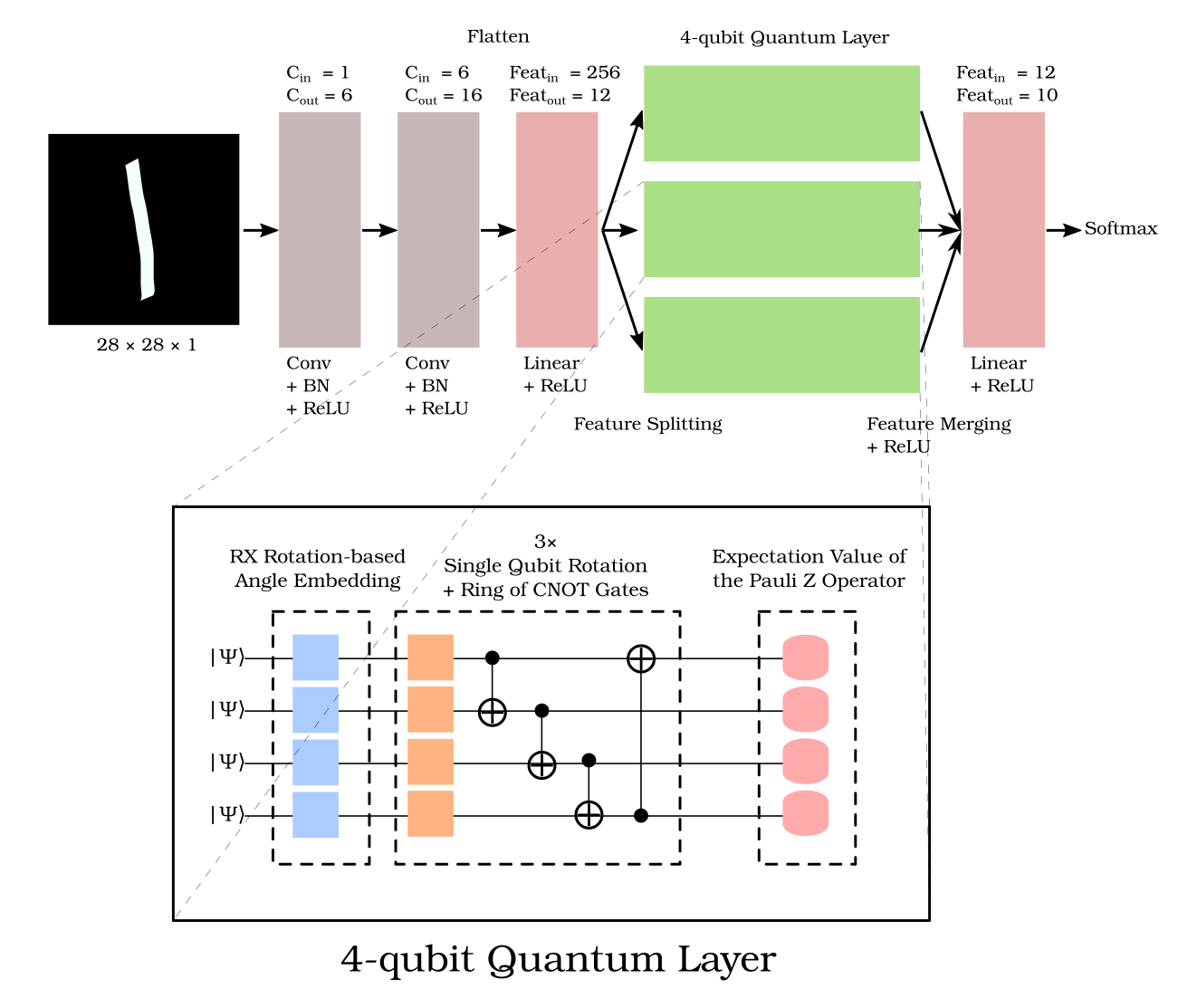 The Quantum LeNet model. The quantum layer consists of embedding, quantum circuits, and measurement.
Quantum computing has shaped our future hope of accomplishing calculations one million times faster than before. Its uses have influenced many things, including machine learning. Such collaboration, known as quantum machine learning (QML), has allowed quantum computers to perform a variety of machine learning tasks. In this project, we will look at how a quantum-based deep-learning model performs image classification on the MNIST dataset. The quantum-based model is a combination of classical and quantum layers. The model is based on LeNet and includes a quantum fully connected layer. The classical and quantum layers are implemented using PyTorch and PennyLane, respectively. This project’s source code is hosted on GitHub.
Quantum Transfer Learning for Lymph Node Metastases Detection
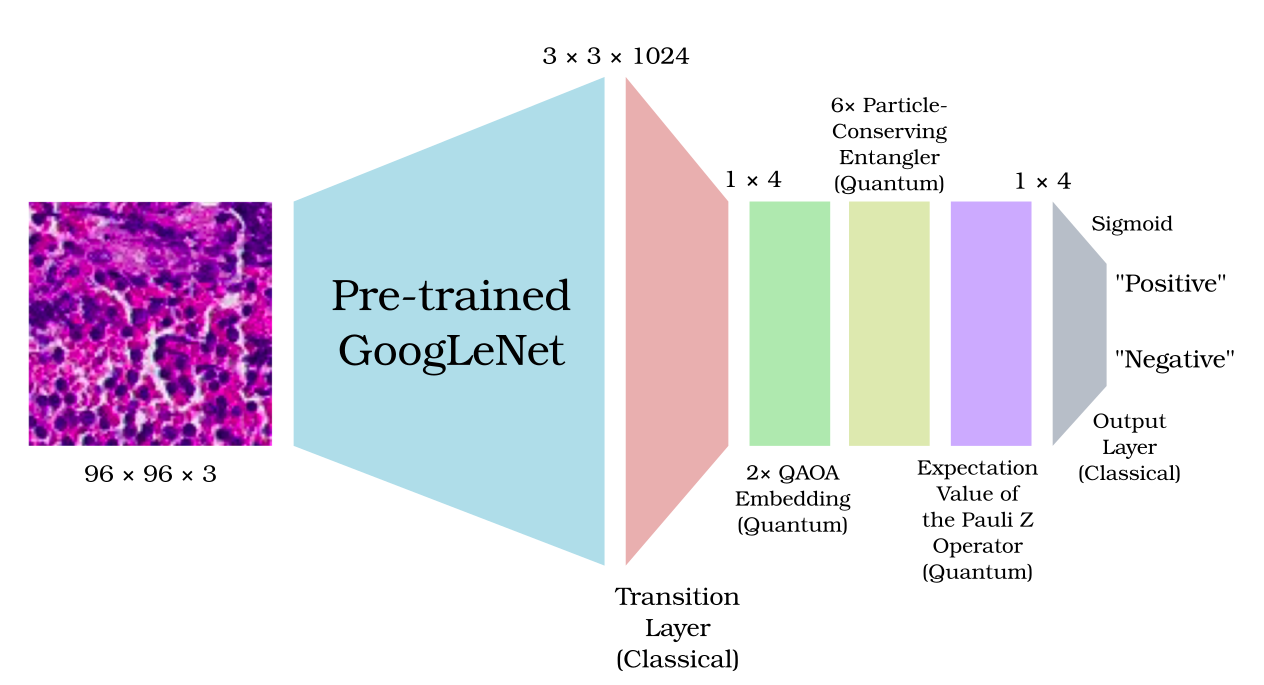 The Quantum GoogLeNet model. The quantum layer: the QAOA-inspired ansatz embedding, the particle-conserving entangler, and the expectation value of the Pauli Z operator.
Transfer learning may make training on a particularly distinguishable dataset easier. It enables several elements of a pre-trained model to be used as the foundation of a new model’s architecture. More importantly, we can adopt this approach in quantum machine learning as well. In this project, we seek to implement quantum transfer learning using an ImageNet-pre-trained model, which will be used on the PCam dataset to tackle the lymph node metastases detection problem. The pre-trained model is GoogLeNet (i.e., Inception V1), and the classifier uses hybrid classical-quantum fully connected layers. Typically, quantum layers are made up of embedding, quantum circuits, and measurement. The embedding and quantum circuits are built upon the QAOA-inspired ansatz and particle-conserving entangler, respectively. This project’s source code is hosted on GitHub.
Other Open Source Software
For a list of my open-source software, please take a look at my GitHub.
